Study › Amateur Extra › E9B

E9B

ANTENNAS AND TRANSMISSION LINES

Antenna patterns and designs: azimuth and elevation patterns; gain as a function of pattern; antenna modeling

Drill results are kept in this browser. Log in to keep them on your account and get a study plan.

E9B011 of 11

What is the 3 dB beamwidth of the antenna radiation pattern shown in Figure E9-1?
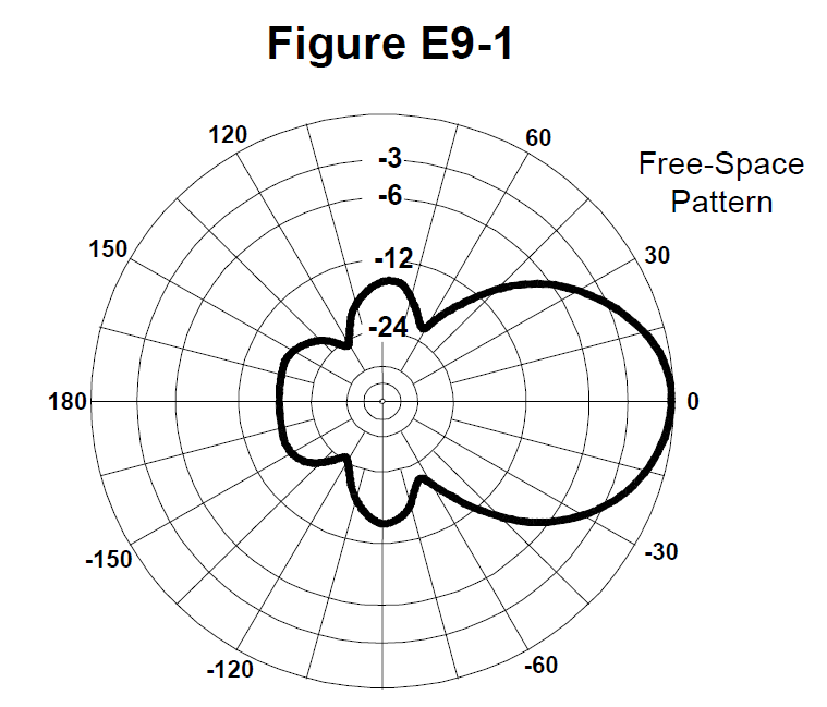
Figure E9-1 from the NCVEC question pool
Why The 3 dB beamwidth is the total angular width of the main lobe measured between the two points where the radiated power has fallen to half (3 dB below) the peak value. On Figure E9-1 you locate the peak of the major lobe, step in one ring to the 3 dB down circle, and read the bearing where the pattern crosses it on each side of the peak. Those crossings are about 25 degrees either side of the lobe axis, so the full beamwidth is 50 degrees.
Watch out The choice saying 25 degrees is the half-beamwidth, the angle from the lobe center out to one 3 dB point, not the width between both points; 75 degrees is closer to where the pattern has dropped much further down, near the lobe edges or nulls.
Beamwidth spans both sides of the peak: find one 3 dB point, then double the angle.
HamSandwich explanation, first draft. The question and answers are the NCVEC text.
E9B022 of 11

What is the front-to-back ratio of the antenna radiation pattern shown in Figure E9-1?

Figure E9-1 from the NCVEC question pool
Why Front-to-back ratio is the difference in dB between the peak of the main lobe and the response exactly 180 degrees behind it. On Figure E9-1 the main lobe peaks at the outer 0 dB ring at the top of the plot, and the small rear lobe at the bottom (180 degrees) reaches in to the ring marked -18 dB, so the ratio is 18 dB. Read the scale rings, not the physical size of the lobes, since polar plots are logarithmic.
Watch out The 14 dB figure is the front-to-side ratio on that same plot, the difference between the main lobe and the response 90 degrees off the front, which a different question in this group asks about.
Front-to-back = straight down from the peak, 180 degrees away. Side lobes at 90 degrees give front-to-side instead.
HamSandwich explanation, first draft. The question and answers are the NCVEC text.
E9B033 of 11

What is the front-to-side ratio of the antenna radiation pattern shown in Figure E9-1?

Figure E9-1 from the NCVEC question pool
Why Front-to-side ratio is read off the polar plot by comparing the peak of the main lobe with the response at 90 degrees away from it. In Figure E9-1 the main lobe peak sits on the outer 0 dB ring, and at the 90 and 270 degree points the pattern has fallen to about the 14 dB ring, so the ratio is roughly 14 dB. The rings on these plots are calibrated in dB below the maximum, so you simply count down from the outer edge to where the trace crosses the side direction.
Watch out The choice that says 18 dB is the front-to-back ratio of this same pattern, measured at 180 degrees from the main lobe, not at the sides.
Same figure, three numbers: 18 dB back, 14 dB side, 50 degree beamwidth. Side is less than back.
HamSandwich explanation, first draft. The question and answers are the NCVEC text.
E9B044 of 11

What is the front-to-back ratio of the radiation pattern shown in Figure E92?

Why Front-to-back ratio compares the main lobe's peak response with the response exactly 180 degrees behind it. On Figure E9-2 the main lobe peak is set on the outer ring, the 0 dB reference, and the small lobe pointing straight down at 180 degrees reaches only the ring 28 dB below that, so the difference is 28 dB. You read the value by counting the dB rings between the two points, not by measuring any physical distance on the paper.
Watch out The choice near 15 dB comes from reading the pattern at 90 degrees off the main lobe, which is the front-to-side ratio, and 3 dB is the half-power level used to find beamwidth, not a lobe ratio.
Front-to-back = straight across the plot, 0 vs 180 degrees. Front-to-side = 90 degrees off.
HamSandwich explanation, first draft. The question and answers are the NCVEC text.
E9B055 of 11

What type of antenna pattern is shown in Figure E9-2?
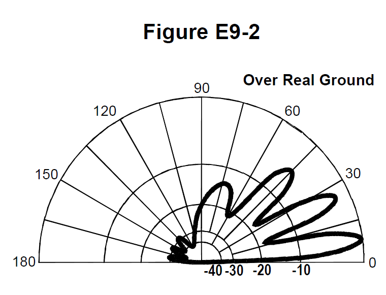
Figure E9-2 from the NCVEC question pool
Why Figure E9-2 plots the radiation in a vertical plane: the angle scale is measured from the horizon upward, and the lobes are stacked above the ground with a null straight down/along the ground, which is the signature of an elevation (vertical plane) pattern. Reading it gives you things like the takeoff angle of the main lobe (about 7.5 degrees in this figure) and the front-to-back ratio. Antenna modeling programs produce both this vertical slice and a horizontal slice for every antenna.
Watch out An azimuth pattern is the horizontal slice, drawn on a full 360 degree compass rose with degrees of bearing around the rim, not degrees above the horizon; near field and polarization are not plot types at all here.
Degrees measured up from the horizon = elevation; degrees around a compass = azimuth.
HamSandwich explanation, first draft. The question and answers are the NCVEC text.
E9B066 of 11

What is the elevation angle of peak response in the antenna radiation pattern shown in Figure E9-2?

Figure E9-2 from the NCVEC question pool
Why Figure E9-2 is an elevation plot: the horizontal line at the left/right edge is the horizon (0 degrees) and angles are measured upward from it toward zenith (90 degrees), with radial grid lines every 15 degrees. The main lobe's maximum lies midway between the horizon and the first 15 degree radial, so the peak response occurs at 7.5 degrees. That low takeoff angle is typical of a horizontal antenna a wavelength or so above real ground, and it is exactly what you want for long-haul DX.
Watch out The choice that says 75 degrees is the same digits transposed and would describe a near-vertical cloud-warmer lobe; 45 degrees is just a grid line well above the main lobe, not its peak.
Elevation angles are measured up from the horizon; the grid is 15 degrees per line, and this lobe peaks at half of the first line.
HamSandwich explanation, first draft. The question and answers are the NCVEC text.
E9B077 of 11

What is the difference in radiated power between a lossless antenna with gain and an isotropic radiator driven by the same power?

Why Antenna gain is not amplification; a passive antenna cannot create power. A lossless antenna radiates 100% of the power delivered to it, exactly as a lossless isotropic radiator does. What gain describes is how that same total power is redistributed, concentrated into some directions at the expense of others, so the field is stronger in the main lobe and weaker elsewhere while the integral over the whole sphere stays constant.
Watch out The idea that the directional antenna radiates more power confuses power density in one direction (which does rise by the gain factor) with total radiated power, which cannot exceed what the transmitter supplies.
Gain redistributes, it does not create. Same watts in, same watts out; only the shape of the pattern changes.
HamSandwich explanation, first draft. The question and answers are the NCVEC text.
E9B088 of 11

What is the far field of an antenna?

Why Close to an antenna, in the reactive near field and the radiating near field (Fresnel region), the relative distribution of energy is still changing as you move outward, so a pattern measured there depends on how far away you are. Beyond a transition distance, commonly estimated as 2D squared divided by wavelength where D is the largest antenna dimension, the wavefront is essentially spherical and the relative pattern shape stays the same while absolute field strength simply falls off as 1/distance. That region is the far field, and it is where gain and radiation patterns are meaningfully specified and where modeling software reports its plots.
Watch out The idea that field strength is constant is backwards: in the far field the field strength keeps decreasing with distance (power density as 1/r squared), and it is only the shape of the pattern, not its magnitude, that stops changing.
Far field = pattern SHAPE frozen, strength still fading. Rough boundary 2D^2 divided by wavelength.
HamSandwich explanation, first draft. The question and answers are the NCVEC text.
E9B099 of 11

What type of analysis is commonly used for modeling antennas?

Why Modern antenna modeling software (NEC, MININEC, EZNEC, 4nec2) is built on the Method of Moments, a numerical technique that breaks the antenna into many short segments, treats the current on each segment as an unknown, and solves the resulting system of simultaneous equations for the currents using the mutual impedances between segments. Once the current distribution is known, the program computes feed point impedance, gain and the azimuth and elevation patterns. It is a numerical approximation, so results depend on using enough segments and on modeling the wires and ground realistically.
Watch out Mutual impedance between elements is one ingredient inside the Method of Moments calculation, not the name of the analysis method itself; graphical and calculus-based approaches are not what antenna modeling programs use.
NEC = Numerical Electromagnetics Code = Method of Moments: chop the wire into segments, solve for the currents.
HamSandwich explanation, first draft. The question and answers are the NCVEC text.
E9B1010 of 11

What is the principle of a Method of Moments analysis?

Why Method of Moments (the math behind NEC-based modeling programs like EZNEC) breaks each wire into many short segments and assumes the current on each segment is constant. The program then builds a matrix of self and mutual impedances between all segments and solves it simultaneously for the current in each one, and those currents give the radiated field, pattern, and feed point impedance. Accuracy depends on using enough segments, typically at least 10 per half wavelength, with segment length short compared to a wavelength.
Watch out The choices about a single sine-wave generator or voltage source describe the old textbook assumption of a sinusoidal current distribution on a dipole, which is an approximation MoM does not need; the voltage-per-segment wording inverts what the model actually solves for, which is current.
Moments = many segments, each carrying one current value. Think 'chop the wire, solve the currents.'
HamSandwich explanation, first draft. The question and answers are the NCVEC text.
E9B1111 of 11

What is a disadvantage of decreasing the number of wire segments in an antenna model below 10 segments per half-wavelength?

Why Method-of-moments programs like NEC approximate the continuous current distribution on a wire by a series of short straight segments, each carrying an assumed simple current. Accuracy depends on having enough segments to follow the sinusoidal current taper, and the accepted rule of thumb is at least 10 segments per half wavelength. With too few segments the current near the source is poorly represented, and since feed point impedance is computed from the voltage and current right at the source segment, the calculated R and X can be significantly off.
Watch out Ground modeling is a separate part of the calculation (the ground model and conductivity/dielectric values you enter), not a function of wire segmentation; harmonic radiation and mechanical strength are physical antenna properties a model does not determine at all.
Remember 10 segments per half wave; too few segments, and the number you can't trust is the feed point impedance.
HamSandwich explanation, first draft. The question and answers are the NCVEC text.
Baofeng BF-F8HP Pro Dual Band HandheldSponsored · View on Amazon →Yaesu FT-65R VHF/UHF Dual Band HandheldSponsored · View on Amazon →
← E9A All groups E9C →